Si in FCC Ni
Based on data in hdl.handle.net/11115/239, “Data Citation: Diffusion of Si impurities in Ni under stress: A first-principles study” by T. Garnier, V. R. Manga, P. Bellon, and D. R. Trinkle (2014). The transport coefficient results, using the self-consistent mean-field method, appear in T. Garnier, V. R. Manga, D. R. Trinkle, M. Nastar, and P. Bellon, “Stress-induced anisotropic diffusion in alloys: Complex Si solute flow near a dislocation core in Ni,” Phys. Rev. B 88, 134108 (2013), doi:10.1103/PhysRevB.88.134108.
[1]:
import sys
sys.path.append('../')
import numpy as np
import matplotlib.pyplot as plt
plt.style.use('seaborn-whitegrid')
%matplotlib inline
import onsager.crystal as crystal
import onsager.OnsagerCalc as onsager
from scipy.constants import physical_constants
kB = physical_constants['Boltzmann constant in eV/K'][0]
import h5py, json
Create an FCC Ni crystal.
[2]:
a0 = 0.343
Ni = crystal.Crystal.FCC(a0, chemistry="Ni")
print(Ni)
#Lattice:
  a1 = [ 0.      0.1715  0.1715]
  a2 = [ 0.1715  0.      0.1715]
  a3 = [ 0.1715  0.1715  0.    ]
#Basis:
  (Ni) 0.0 = [ 0.  0.  0.]
Next, we construct our diffuser. For this problem, our thermodynamic range is out to the fourth neighbor; hence, we construct a two shell thermodynamic range (that is, sums of two \(\frac{a}{2}\langle 110\rangle\) vectors. That is, \(N_\text{thermo}=2\) gives 4 stars: \(\frac{a}2\langle110\rangle\), \(a\langle100\rangle\), \(\frac{a}2\langle112\rangle\), and \(a\langle110\rangle\). For Si in Ni, the first three have non-zero interaction energies, while the fourth is zero. The states, as written, are the solute (basis index + lattice position) : vacancy (basis index + lattice position), and \(dx\) is the (Cartesian) vector separating them.
[3]:
chemistry = 0 # only one sublattice anyway
Nthermo = 2
NiSi = onsager.VacancyMediated(Ni, chemistry, Ni.sitelist(chemistry),
                               Ni.jumpnetwork(chemistry, 0.75*a0), Nthermo)
print(NiSi)
Diffuser for atom 0 (Ni), Nthermo=2
#Lattice:
  a1 = [ 0.      0.1715  0.1715]
  a2 = [ 0.1715  0.      0.1715]
  a3 = [ 0.1715  0.1715  0.    ]
#Basis:
  (Ni) 0.0 = [ 0.  0.  0.]
vacancy configurations:
v:+0.000,+0.000,+0.000
solute configurations:
s:+0.000,+0.000,+0.000
solute-vacancy configurations:
s:+0.000,+0.000,+0.000-v:+1.000,-1.000,+0.000
s:+0.000,+0.000,+0.000-v:-1.000,-1.000,+1.000
s:+0.000,+0.000,+0.000-v:+0.000,+1.000,-2.000
s:+0.000,+0.000,+0.000-v:-2.000,+0.000,+0.000
omega0 jumps:
omega0:v:+0.000,+0.000,+0.000^v:+0.000,+0.000,-1.000
omega1 jumps:
omega1:s:+0.000,+0.000,+0.000-v:-1.000,+0.000,+0.000^v:-1.000,+0.000,-1.000
omega1:s:+0.000,+0.000,+0.000-v:+1.000,+0.000,+0.000^v:+1.000,+0.000,-1.000
omega1:s:+0.000,+0.000,+0.000-v:-1.000,+1.000,+0.000^v:-1.000,+1.000,-1.000
omega1:s:+0.000,+0.000,+0.000-v:+0.000,+0.000,-1.000^v:+0.000,+0.000,-2.000
omega1:s:+0.000,+0.000,+0.000-v:+1.000,-1.000,-1.000^v:+1.000,-1.000,-2.000
omega1:s:+0.000,+0.000,+0.000-v:-1.000,-1.000,+1.000^v:-1.000,-1.000,+0.000
omega1:s:+0.000,+0.000,+0.000-v:-1.000,+0.000,-1.000^v:-1.000,+0.000,-2.000
omega1:s:+0.000,+0.000,+0.000-v:-2.000,+1.000,+0.000^v:-2.000,+1.000,-1.000
omega1:s:+0.000,+0.000,+0.000-v:+1.000,+1.000,-2.000^v:+1.000,+1.000,-3.000
omega1:s:+0.000,+0.000,+0.000-v:+2.000,+0.000,-1.000^v:+2.000,+0.000,-2.000
omega1:s:+0.000,+0.000,+0.000-v:-2.000,+1.000,+1.000^v:-2.000,+1.000,+0.000
omega1:s:+0.000,+0.000,+0.000-v:-2.000,+0.000,+0.000^v:-2.000,+0.000,-1.000
omega1:s:+0.000,+0.000,+0.000-v:+2.000,-2.000,+0.000^v:+2.000,-2.000,-1.000
omega1:s:+0.000,+0.000,+0.000-v:+0.000,+0.000,-2.000^v:+0.000,+0.000,-3.000
omega2 jumps:
omega2:s:+0.000,+0.000,+0.000-v:+0.000,+0.000,+1.000^s:+0.000,+0.000,+0.000-v:+0.000,+0.000,-1.000
Below is an example of the above data translated into a dictionary corresponding to the data for Ni-Si; it is output into a JSON compliant file for reference. The strings are the corresponding tags in the diffuser. The first entry in each list is the prefactor (in THz) and the second is the corresponding energy (in eV). Note: all jumps are defined as transition state energies, hence the reference energy is added / subtracted as needed. Also, there are “missing” transition states; these
will have there energies defined using the LIMB (linear interpolation of migration barriers) approximation. This introduces an error of no more than 10 meV in any activation barrier.
[4]:
NiSidata={
"v:+0.000,+0.000,+0.000": [1., 0.],
"s:+0.000,+0.000,+0.000": [1., 0.],
"s:+0.000,+0.000,+0.000-v:+0.000,+1.000,-1.000": [1., -0.108],
"s:+0.000,+0.000,+0.000-v:-1.000,-1.000,+1.000": [1., +0.004],
"s:+0.000,+0.000,+0.000-v:+1.000,-2.000,+0.000": [1., +0.037],
"s:+0.000,+0.000,+0.000-v:+0.000,-2.000,+0.000": [1., -0.008],
"omega0:v:+0.000,+0.000,+0.000^v:+0.000,+1.000,-1.000": [4.8, 1.074],
"omega1:s:+0.000,+0.000,+0.000-v:-1.000,+0.000,+0.000^v:-1.000,+1.000,-1.000": [5.2, 1.213-0.108],
"omega1:s:+0.000,+0.000,+0.000-v:+0.000,-1.000,+0.000^v:+0.000,+0.000,-1.000": [5.2, 1.003-0.108],
"omega1:s:+0.000,+0.000,+0.000-v:+0.000,+1.000,-1.000^v:+0.000,+2.000,-2.000": [4.8, 1.128-0.108],
"omega1:s:+0.000,+0.000,+0.000-v:-1.000,+1.000,+0.000^v:-1.000,+2.000,-1.000": [5.2, 1.153-0.108],
"omega1:s:+0.000,+0.000,+0.000-v:+1.000,-1.000,-1.000^v:+1.000,+0.000,-2.000": [4.8, 1.091+0.004],
"omega2:s:+0.000,+0.000,+0.000-v:+0.000,-1.000,+1.000^s:+0.000,+0.000,+0.000-v:+0.000,+1.000,-1.000": [5.1, 0.891-0.108]
}
NiSi2013data={
"v:+0.000,+0.000,+0.000": [1., 0.],
"s:+0.000,+0.000,+0.000": [1., 0.],
"s:+0.000,+0.000,+0.000-v:+0.000,+1.000,-1.000": [1., -0.100],
"s:+0.000,+0.000,+0.000-v:-1.000,-1.000,+1.000": [1., +0.011],
"s:+0.000,+0.000,+0.000-v:+1.000,-2.000,+0.000": [1., +0.045],
"s:+0.000,+0.000,+0.000-v:+0.000,-2.000,+0.000": [1., 0],
"omega0:v:+0.000,+0.000,+0.000^v:+0.000,+1.000,-1.000": [4.8, 1.074],
"omega1:s:+0.000,+0.000,+0.000-v:-1.000,+0.000,+0.000^v:-1.000,+1.000,-1.000": [5.2, 1.213-0.100],
"omega1:s:+0.000,+0.000,+0.000-v:+0.000,-1.000,+0.000^v:+0.000,+0.000,-1.000": [5.2, 1.003-0.100],
"omega1:s:+0.000,+0.000,+0.000-v:+0.000,+1.000,-1.000^v:+0.000,+2.000,-2.000": [4.8, 1.128-0.100],
"omega1:s:+0.000,+0.000,+0.000-v:-1.000,+1.000,+0.000^v:-1.000,+2.000,-1.000": [5.2, 1.153-0.100],
"omega1:s:+0.000,+0.000,+0.000-v:+1.000,-1.000,-1.000^v:+1.000,+0.000,-2.000": [4.8, 1.091+0.011],
"omega2:s:+0.000,+0.000,+0.000-v:+0.000,-1.000,+1.000^s:+0.000,+0.000,+0.000-v:+0.000,+1.000,-1.000": [5.1, 0.891-0.100]
}
print(json.dumps(NiSi2013data, sort_keys=True, indent=4))
{
    "omega0:v:+0.000,+0.000,+0.000^v:+0.000,+1.000,-1.000": [
        4.8,
        1.074
    ],
    "omega1:s:+0.000,+0.000,+0.000-v:+0.000,+1.000,-1.000^v:+0.000,+2.000,-2.000": [
        4.8,
        1.0279999999999998
    ],
    "omega1:s:+0.000,+0.000,+0.000-v:+0.000,-1.000,+0.000^v:+0.000,+0.000,-1.000": [
        5.2,
        0.9029999999999999
    ],
    "omega1:s:+0.000,+0.000,+0.000-v:+1.000,-1.000,-1.000^v:+1.000,+0.000,-2.000": [
        4.8,
        1.1019999999999999
    ],
    "omega1:s:+0.000,+0.000,+0.000-v:-1.000,+0.000,+0.000^v:-1.000,+1.000,-1.000": [
        5.2,
        1.113
    ],
    "omega1:s:+0.000,+0.000,+0.000-v:-1.000,+1.000,+0.000^v:-1.000,+2.000,-1.000": [
        5.2,
        1.053
    ],
    "omega2:s:+0.000,+0.000,+0.000-v:+0.000,-1.000,+1.000^s:+0.000,+0.000,+0.000-v:+0.000,+1.000,-1.000": [
        5.1,
        0.791
    ],
    "s:+0.000,+0.000,+0.000": [
        1.0,
        0.0
    ],
    "s:+0.000,+0.000,+0.000-v:+0.000,+1.000,-1.000": [
        1.0,
        -0.1
    ],
    "s:+0.000,+0.000,+0.000-v:+0.000,-2.000,+0.000": [
        1.0,
        0
    ],
    "s:+0.000,+0.000,+0.000-v:+1.000,-2.000,+0.000": [
        1.0,
        0.045
    ],
    "s:+0.000,+0.000,+0.000-v:-1.000,-1.000,+1.000": [
        1.0,
        0.011
    ],
    "v:+0.000,+0.000,+0.000": [
        1.0,
        0.0
    ]
}
Next, we convert our dictionary into the simpler form used by the diffuser.
[5]:
preenedict = NiSi.tags2preene(NiSi2013data)
preenedict
[5]:
{'eneS': array([ 0.]),
 'eneSV': array([-0.1  ,  0.011,  0.045,  0.   ]),
 'eneT0': array([ 1.074]),
 'eneT1': array([ 1.053 ,  0.903 ,  1.113 ,  1.028 ,  1.0795,  1.102 ,  1.0965,
         1.0965,  1.0965,  1.0965,  1.119 ,  1.074 ,  1.074 ,  1.074 ]),
 'eneT2': array([ 0.791]),
 'eneV': array([ 0.]),
 'preS': array([ 1.]),
 'preSV': array([ 1.,  1.,  1.,  1.]),
 'preT0': array([ 4.8]),
 'preT1': array([ 5.2,  5.2,  5.2,  4.8,  4.8,  4.8,  4.8,  4.8,  4.8,  4.8,  4.8,
         4.8,  4.8,  4.8]),
 'preT2': array([ 5.1]),
 'preV': array([ 1.])}
We can now calculate the diffusion coefficients and drag ratio. Note: the diffusion coefficients \(L_\text{ss}\) and \(L_\text{sv}\) both need to be multiplied by \(c_\text{s}c_\text{v}/k_\text{B}T\) where \(c_\text{s}\) is the solute concentration, \(c_\text{v}\) the (equilibrium) vacancy concentration, and \(k_\text{B}T\) is the thermal energy of the system. The current units shown below are in \(\text{nm}^2\cdot\text{THz}\).
[6]:
print("#T #Lss #Lsv #drag")
for T in np.linspace(300, 1400, 23):
    L0vv, Lss, Lsv, L1vv = NiSi.Lij(*NiSi.preene2betafree(kB*T, **preenedict))
    print(T, Lss[0,0], Lsv[0,0], Lsv[0,0]/Lss[0,0])
#T #Lss #Lsv #drag
300.0 4.1020388689e-16 4.03521345382e-16 0.983709219436
350.0 5.99654580387e-14 5.75933473853e-14 0.960442048956
400.0 2.51914470587e-12 2.32702939103e-12 0.923737880405
450.0 4.61249420384e-11 4.03116417036e-11 0.873966230027
500.0 4.7250491963e-10 3.84170227063e-10 0.813050216206
550.0 3.17382569388e-09 2.36031280433e-09 0.743680665541
600.0 1.55354740581e-08 1.03884191885e-08 0.668690195716
650.0 5.96097883468e-08 3.52092669306e-08 0.590662505388
700.0 1.88868586771e-07 9.66525181976e-08 0.511744805477
750.0 5.13340570374e-07 2.22584238868e-07 0.43359954719
800.0 1.23159242387e-06 4.40215392835e-07 0.357435937654
850.0 2.66586838346e-06 7.57314596438e-07 0.28407801418
900.0 5.29556637614e-06 1.13347630469e-06 0.214042507294
950.0 9.78435004446e-06 1.44428949825e-06 0.147612206399
1000.0 1.69973273335e-05 1.44304978386e-06 0.084898628799
1050.0 2.80063788635e-05 7.25153043356e-07 0.0258924242542
1100.0 4.4083410105e-05 -1.3003604007e-06 -0.0294977270951
1150.0 6.66826933232e-05 -5.4290391372e-06 -0.0814160146604
1200.0 9.74143994545e-05 -1.26676005168e-05 -0.130038275529
1250.0 0.000138011882666 -2.42289344792e-05 -0.175556872431
1300.0 0.000190295346612 -4.15167679854e-05 -0.21817016929
1350.0 0.000256134304169 -6.61019634203e-05 -0.258075401632
1400.0 0.000337410855954 -9.96927651132e-05 -0.295464011765
For direct comparison with the SCMF data in the 2013 Phys. Rev. B paper, we evaluate at 960K, 1060K (the predicted crossover temperature), and 1160K. The reported data is in units of mol/eV Å ns.
[7]:
volume = 0.25*a0**3
conv = 1e3*0.1/volume  # 10^3 for THz->ns^-1, 10^-1 for nm^-1 ->Ang^-1
# T: (L0vv, Lsv, Lss)
PRBdata = {960: (1.52e-1, 1.57e-1, 1.29e0),
           1060: (4.69e-1, 0., 3.27e0),
           1160: (1.18e0, -7.55e-1, 7.02e0)}
print("#T #Lvv #Lsv #Lss")
for T in (960, 1060, 1160):
    c = conv/(kB*T)
    L0vv, Lss, Lsv, L1vv = NiSi.Lij(*NiSi.preene2betafree(kB*T, **preenedict))
    vv, sv, ss = L0vv[0,0]*c, Lsv[0,0]*c, Lss[0,0]*c
    vvref, svref, ssref = PRBdata[T]
    print("{} {:.4g} ({:.4g}) {:.4g} ({:.4g}) {:.4g} ({:.4g})".format(T, vv, vvref/vv, sv, svref/sv, ss, ssref/ss))
#T #Lvv #Lsv #Lss
960 0.1556 (0.9766) 0.1773 (0.8856) 1.315 (0.9807)
1060 0.4797 (0.9777) 0.04852 (0) 3.339 (0.9792)
1160 1.208 (0.9769) -0.6537 (1.155) 7.152 (0.9815)
[8]:
# raw comparison data from 2013 paper
Tval = np.array([510, 530, 550, 570, 590, 610, 630, 650, 670, 690,
                 710, 730, 750, 770, 790, 810, 830, 850, 870, 890,
                 910, 930, 950, 970, 990, 1010, 1030, 1050, 1070, 1090,
                 1110, 1130, 1150, 1170, 1190, 1210, 1230, 1250, 1270, 1290,
                 1310, 1330, 1350, 1370, 1390, 1410, 1430, 1450, 1470, 1490])
fluxval = np.array([0.771344, 0.743072, 0.713923, 0.684066, 0.653661, 0.622858,
                    0.591787, 0.560983, 0.529615, 0.498822, 0.467298, 0.436502,
                    0.406013, 0.376193, 0.346530, 0.316744, 0.288483, 0.260656,
                    0.232809, 0.205861, 0.179139, 0.154038, 0.128150, 0.103273,
                    0.079025, 0.055587, 0.032558, 0.010136, -0.011727, -0.033069,
                    -0.053826, -0.074061, -0.093802, -0.113075, -0.132267, -0.149595,
                    -0.167389, -0.184604, -0.202465, -0.218904, -0.234157, -0.250360,
                    -0.265637, -0.280173, -0.294940, -0.308410, -0.322271, -0.335809,
                    -0.349106, -0.361605])
# Trange = np.linspace(300, 1500, 121)
Draglist = []
for T in Tval:
    L0vv, Lss, Lsv, L1vv = NiSi.Lij(*NiSi.preene2betafree(kB*T, **preenedict))
    Draglist.append(Lsv[0,0]/Lss[0,0])
Drag = np.array(Draglist)
[9]:
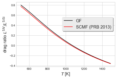
fig, ax1 = plt.subplots()
ax1.plot(Tval, Drag, 'k', label='GF')
ax1.plot(Tval, fluxval, 'r', label='SCMF (PRB 2013)')
ax1.set_ylabel('drag ratio $L^{\\rm{SiV}}/L^{\\rm{SiSi}}$', fontsize='x-large')
ax1.set_xlabel('$T$ [K]', fontsize='x-large')
ax1.legend(bbox_to_anchor=(0.5,0.6,0.5,0.2), ncol=1,
           shadow=True, frameon=True, fontsize='x-large')
plt.show()
# plt.savefig('NiSi-drag.pdf', transparent=True, format='pdf')